Feature selection with Lasso Regularization Path
In a nutshell
Imagine you’re a chef in a kitchen full of ingredients, some of which enhance your dish’s flavor, while others might not blend well together or might even spoil the taste.
In the world of data analysis, this culinary challenge is akin to feature selection — the art of choosing the right set of ingredients (predictors) to make your model (dish) as predictive and understandable as possible.
Among various techniques to select features, Lasso regularization path is my personal favorite:
- it has solid statistical foundations
- we can base it on information criterions
- it has a very visual interpretation
In this post we will see how to get an explainable, criterion based feature selection from a Lasso regressor, by incrementally decreasing its \(l_1\) penalty
What is Feature Selection
When you come across a “traditional” statistical modeling (regression/classification), feature selection emerges as a critical process. This technique is about identifying the most impactful predictors for your model. The ideal set of features accomplishes two main objectives:
- Inclusion of Predictive Variables: It consists of predictors that either independently or in combination with others, significantly explain variance in the target outcome.
- Exclusion of Redundant Variables: It avoids predictors that are inter-correlated, known as having collinearity, which can distort the model’s performance and interpretability.
Why is it Important?
The importance of feature selection extends beyond mere model simplification. It directly prevents overfitting, ensuring the model’s generalizability to unseen data. Moreover, by narrowing down the predictors to a core set, it enhances the model’s interpretability.
Despite its significance, feature selection often doesn’t receive the attention it deserves, particularly in scenarios where:
Data Abundance: With more variables \(p\) than observations \(n\), it is tempting to keep all available data, hoping the model will sort it out.
Model Resilience: Certain models claim to handle co-linearity well. While this might be true to an extent, relying solely on this capability can sometimes obscure the true relationships in your data.
However, this may result in a suboptimal/overfitted model, particularly if it’s the initial strategy employed. The benefits of a carefully curated feature set are significant. It not only aids in a deeper comprehension of the fundamental relationships within your data but also helps illuminate the core business principles guiding these interactions.
There is a time to understand data and build explainable models, and a time to build accurate models.
Lasso Regression
The \(\lambda\) penalty
The Lasso (Least Absolute Shrinkage and Selection Operator) is a type of linear regression, that notably uses a regularization term in the form of a \(l_1\) penalty. (i.e. euclidian norm).
Lasso objective is to solve
\[\underset{\beta_0, \beta}{\text{min}} \Bigl\{ \sum_{i=1}^{n}(y_i - \beta_0 - x_i^T\beta)^2 \Bigr\}, \text{with} \sum_{j=1}^{p}| \beta_j| \leq \lambda\]With
- \(y\) the outcome vector (values to predict)
- \(x\) the feature vector (features available)
- \(\beta_0\) the intercept
- \(\beta=(\beta_1, \ldots, \beta_p)\) coefficients associated with each feature
- we can denote \(\hat{y} = \beta_0 - x^T\beta\) the predicted values
It means that it has to adapt its coefficients \(\beta\) to minimize the square of the residual errors \((y - \hat{y})^2\), but under the additional constraint that the sum of coefficients absolute value must not exceed a fixed and arbitrary limit \(\lambda\) (sometimes noted \(t\)).
Consider that your target and features are scaled to the same interval at this point
Basically, you are not asking your model to accurately predict \(y\) anymore (it won’t), the objective is now more:
“If you were to get stranded on a deserted island, with a backpack of size \(f(\lambda)\), what features are you bringing with you?”
Understanding the Impact of Lambda
Low Lambda: A smaller \(\lambda\) increases the penalty, leading to more coefficients being shrunk to zero. This simplifies the model but may also lead to underfitting.
High Lambda: A larger \(\lambda\) means less penalty on the coefficients. This can lead to a model similar to a standard linear regression, potentially causing overfitting if there are many predictors.
Think of it as a feature budget you are giving to the Lasso.
Navigating the Path of Regularization
The regularization path consists in gradually changing the value of the regularization parameter \(\lambda\) and observing how this affects the model coefficients. As \(\lambda\) increases, more coefficients are driven to zero, effectively eliminating variables from the model.
But, my model will perform more and more badly, right?
Right! And quite frankly, we do not really care on how bad it will actually perform at the end. We are giving more interest to the coefficients variation at this time.
Anyway, remember our Lasso is just a linear model that will very likely not compete with non-linear, robust estimators like a Random Forest. That is not our goal at the moment.
Choosing the Right Lambda
One of the primary advantages of utilizing a parameterized estimator like Lasso regression, as opposed to ensemble methods, lies in its capability to straightforwardly estimate the model’s likelihood.
The likelihood of an estimator is essentially the probability of observing the given data under the assumed model, as a function of the model parameters.
This feature grants direct access to powerful tools known as information criteria, specifically Akaike’s Information Criterion (AIC) and the Bayesian Information Criterion (BIC). They differ mainly in their penalty terms; AIC penalizes the complexity less harshly than BIC, making BIC more stringent about model simplicity.
In the context of Lasso regression, these criteria help in striking a balance between model complexity and goodness of fit. Lower values of AIC or BIC indicate a better model choice. The likelihood component of these criteria assesses how probable it is that the model could have produced the observed data.
The true power of using AIC/BIC in conjunction with Lasso lies in their ability to guide the selection of lambda towards a model that is complex enough to capture the underlying patterns in the data, yet simple enough to avoid overfitting.
By minimizing AIC or BIC, one can find an optimal lambda that achieves this balance.
Examples
Before going into the code, let’s illustrate what we explain before with some example datasets.
Wine Quality
Let’s begin with a straightforward example with the Wine Quality Dataset (red subset). The goal is to predict a wine quality, given some chemical properties. All features and target are purely numerical, so there is no need of processing data beyond a scaling.
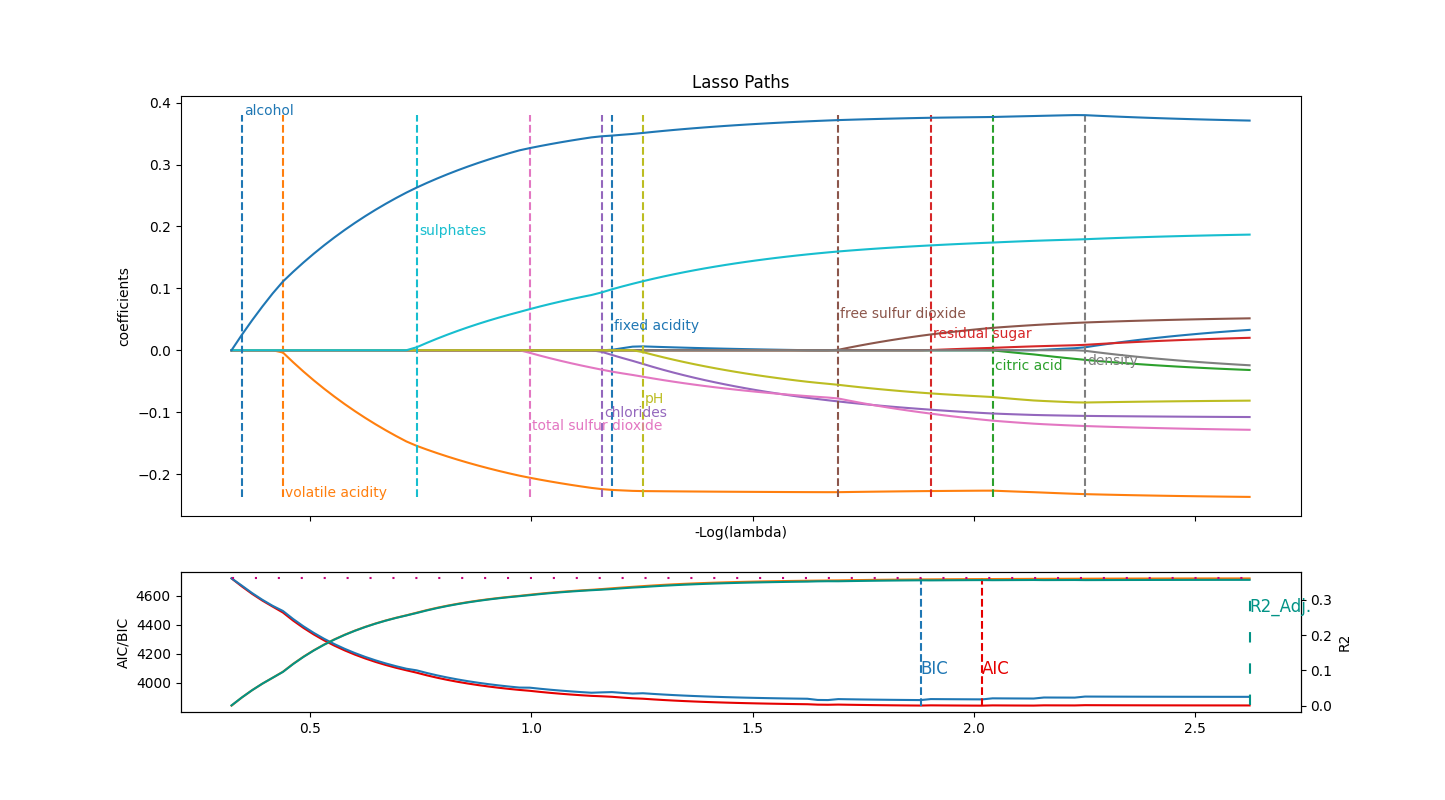
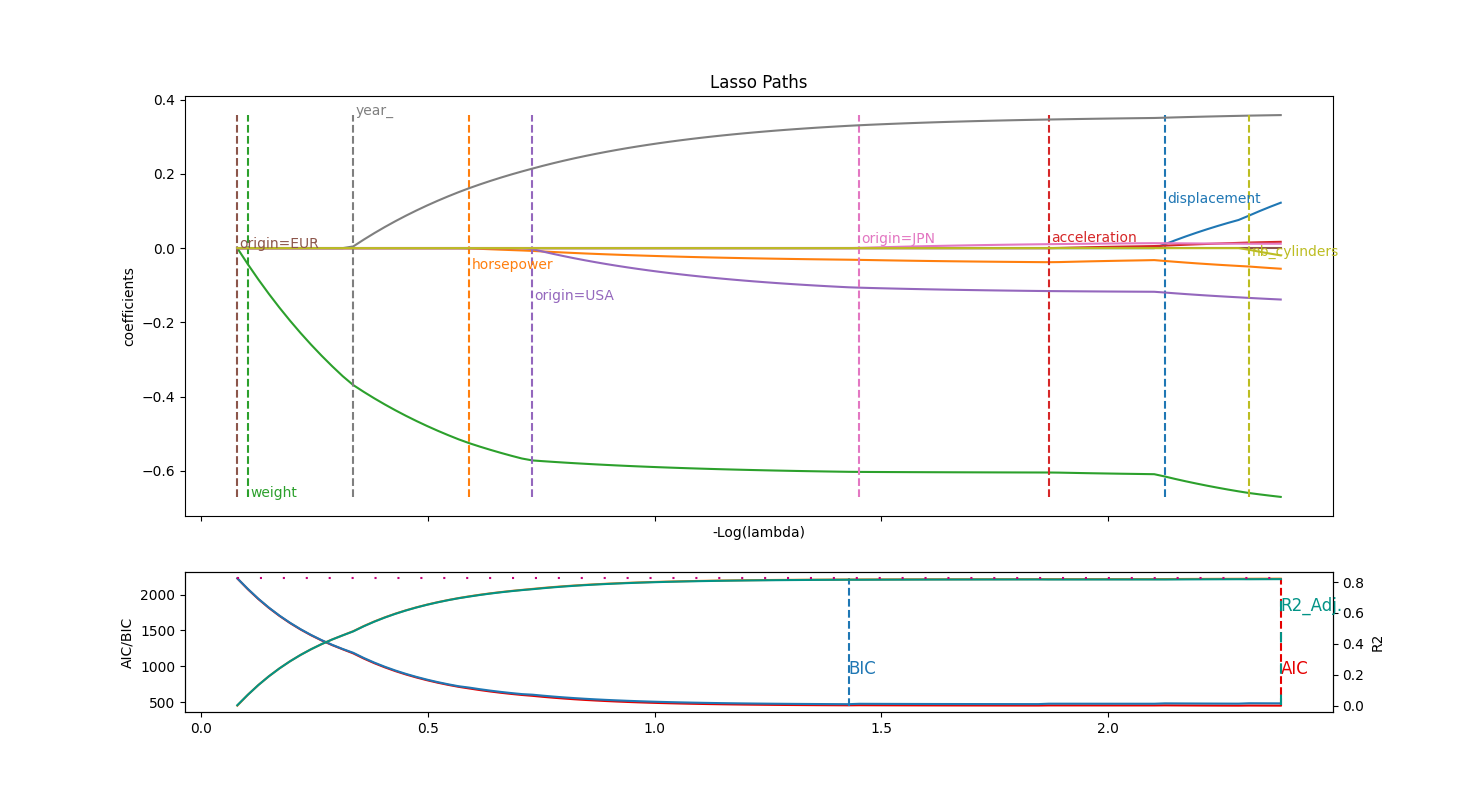
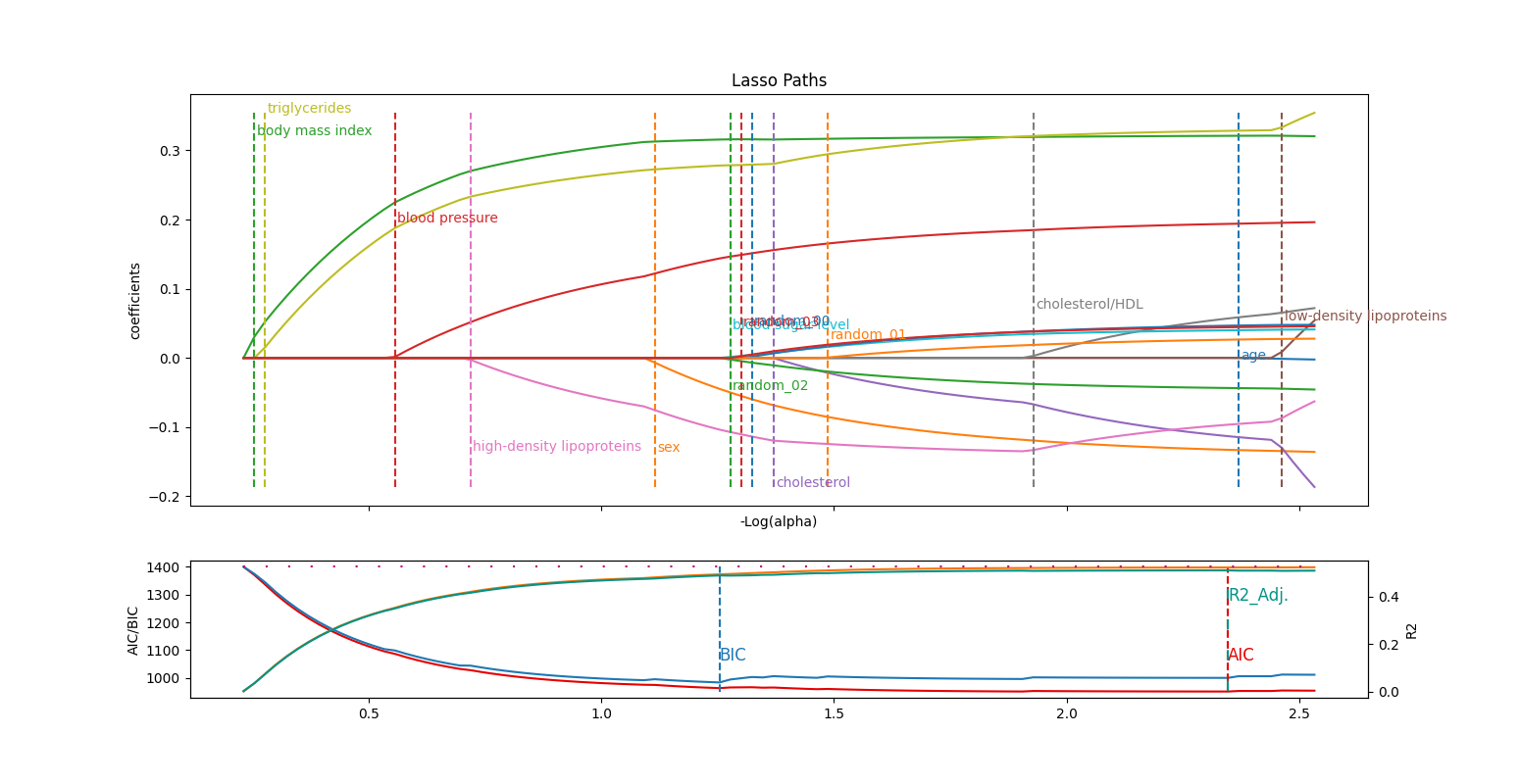
On the first subplot, we plot the regularization path that each features follows, starting from the most simple (restricted) model (left) to the least (right). The final model is basically a standard linear model.
On the second one, we plot the evolution of information criteria for the estimator obtained at that level of regularization, along with the \(R^2\) criterion and its adjusted variant.
What we can say here is that alcolhol has a clear, massive positive influence, while on the contrary volatile_acidity is its negative counterpart. Then sulphates and total sulfur dioxide come into consideration to a lesser extent. fixed_acidity is picked, but discarded soon after as pH probably holds the same information.
BIC criterion admits free_sulfur_dioxyde before closing the feature set, while AIC takes additionnally residual_sugar. Other features are not considered to enrich the model.
Be precautious, as our \(R^2 `simeq 0.35\), which is quite bad while already explaining some of the variance. Some additional feature engineering might be the next step!
Cars comsumption
The goal in this Auto MPG dataset is to predict a car consumption (miles per gallon).purely numeric
The difficulty is to deal with some features that are not continuous but discrete:
year, that we however treat as ordinal, becoming more amodel_youthfeaturecylindersis treated as ordinal as well, actually I do not see the caveat in considering it continuousorigin, that we can treat with one-hot encoding, becoming three distinct features
Good to observe that you reach the same accuracy with 5/9 of available features, discarding three original features. The selected model is actually pretty good with a \(R^2 \simeq 0.80\), indicating that a linear model might be a good approach.
Diabetes
As a last example, we take the diabetes regression dataset from scikit-learn, that depicts the evolution of diabete disease.
1
2
3
4
5
6
7
8
9
10
11
12
13
from sklearn import datasets

X, y = datasets.load_diabetes(return_X_y=True, as_frame=True)

X.columns = [ 'age', 'sex', 'body mass index', 'blood pressure', 'cholesterol', 'low-density lipoproteins','high-density lipoproteins', 'cholesterol/HDL', 'triglycerides', 'blood sugar level']

rng = np.random.RandomState(42)
n_random_features = 4
X_random = pd.DataFrame(
	rng.randn(X.shape[0], n_random_features),
	columns=[f"random_{i:02d}" for i in range(n_random_features)],
)
X = pd.concat([X, X_random], axis=1)
To add a difficulty, we generated 4 random features that do not explain any variance on the target.
Five features (body mass index, triglycerides, blood pressure, high density lipoproteins and sex) stand out significantly in this analysis, being by the magnitude of their respective coefficients and the fact that they are identified individually rather than as part of a large group of variables.
Moreover, the BIC criterion, known for its stricter selection process, exclusively retains these variables. Unlike AIC, which can sometimes incorporate arbitrary features, BIC effectively avoids this pitfall.
Lasso Regression in Practice: A Step-by-Step Guide
- Data Preparation: Begin with standardizing your data. Lasso makes no sense if features are of different orders of magnitude
- Model Building: Implement Lasso regression using libraries in R (like glmnet) or Python (such as scikit-learn).
- Regularization Path Analysis: Plot the path of coefficients against different lambda values to observe how variable selection evolves.
- Optimal Lambda Selection: Use argmin of AIC/BIC to find the best set a features
- Interpreting the Results: Analyze the final model, focusing on the variables that survived the regularization process.
Hands-on with scikit-learn
1
2
3
4
5
6
7
8
9
10
11
12
13
14
15
16
17
18
19
20
21
22
23
24
25
26
27
28
29
30
31
32
33
34
35
36
37
38
39
40
41
42
43
44
45
46
47
48
49
50
51
52
53
54

# criterion on which we will base our model selection (aic/bic/r2/r2_adj)
MODEL = 'bic'

from itertools import cycle

import numpy as np
import pandas as pd

from sklearn.linear_model import lasso_path, enet_path, lars_path, LassoLarsIC, LinearRegression
from sklearn.preprocessing import StandardScaler

from sklearn.pipeline import make_pipeline

import matplotlib.pyplot as plt
import matplotlib._color_data as mcd

def unregularized(X, y):
	"""Compute an estimate of the variance and unregularized R2 with an OLS model.
		Parameters
		----------
		X : ndarray of shape (n_samples, n_features)
			Data to be fitted by the OLS model. We expect the data to be
			centered.
		y : ndarray of shape (n_samples,)
			Associated target.

		Returns
		-------
		noise_variance : float
			An estimator of the noise variance of an OLS model.
	"""
	if X.shape[0] <= X.shape[1] :
		raise ValueError("n < p ")
	# X and y are already centered and we don't need to fit with an intercept
	ols_model = LinearRegression(fit_intercept = False)
	y_pred = ols_model.fit(X, y).predict(X)
	return np.sum((y - y_pred) ** 2) / (X.shape[0] - X.shape[1]), ols_model.score(X, y)

def zou_et_al_criterion_rescaling(criterion, n_samples, noise_variance):
	"""Rescale the information criterion to follow the definition of Zou et al."""
	return criterion - n_samples * np.log(2 * np.pi * noise_variance) - n_samples

def information_criterions_ols(residuals_sum_squares, n_samples, noise_variance_, degrees_of_freedom) :
	criterion_aic = (n_samples * np.log(2 * np.pi * noise_variance_)
				+ residuals_sum_squares / noise_variance_
				+ 2 * degrees_of_freedom)

	criterion_bic = (n_samples * np.log(2 * np.pi * noise_variance_)
				+ residuals_sum_squares / noise_variance_
				+ np.log(n_samples) * degrees_of_freedom)

	return criterion_aic, criterion_bic
1
2
3
4
5
6
7
8
9
10
11
12
13
14
15
16
17
18
19
20
21
22
23
24
25
26
27
28
29
30
31
32
33
34
35
36
37
38
39
40
41
42
43
44
45
46
47
48
49
50
51
52
53
54
55
56
57
58
59
60
61
62
63
64
65
66
67
68
69
70
71
72
73
74
75
76
77
78
79
80
81
82
83
84
85
86
87
88
89
90
91
92
93
94
95
96
97
98
99
100
101
102
103
104
105
106
107
108
109
110
111
112
113
114
115
116
117
118
119
120
121
122
123
124
125
126
127
128
129
130
131
132
133
134
135
136
137
138
139
140
141
142
143
144
145
146
147
148
149
150
151
152
153
154
155
156
157
158
159
160
161
162
163
164
165
166
167
168
169
170
171
172
173
174
175
176
177
178
179
180
181
182
183
184
185
186
187
188
189
190
191
192
193
def regularization_path(X, y, feature_names, model = 'lasso', scale = False, l1_ratio=0.5, eps = 5e-3, plot = True, zou_rescale = False):
	"""
	Trains several linear models with an increasing penalty L1 (Lasso) or L1/L2 (Elastic Net).
	The goal is to select variables according to their coefficient variation towards this regularization.
		-> Variables which are selected at first and stay high are important
		-> Variables which are only selected at the end and at a small coeff are probably not relevant
		-> Conjugate moves between 2 or more variables is a colinearity indicator ; achtung !

	Note : Only use at selection step, an unrestricted model should be preferred for actual modelling.

	Parameters :
		X (np.array(n,p))
		y (np.array(n,))
		model (str in {'lasso', 'enet', 'lars'}) : Lasso Regression (Pure L1 penalty) or Elastic Net (mix of L1/L2 penalty)
		l1_ratio (float=0.5) : only used with enet, ratio of l1 penalty
		eps (float=5e-3) : the smaller it is the longer is the path
		plot (bool) : wether to plot or not paths figure
		zou_rescale (bool=False) : AIC/BIC rescaling according to Zou et al.

	Returns:
		df_reg (pandas DataFrame) :
			row is a model corresponding to an eps value,
			cols are coefs affected to respective X for that model

	Example :
from sklearn import datasets

X, y = datasets.load_diabetes(return_X_y=True, as_frame=True)

rng = np.random.RandomState(42)
n_random_features = 4
X.columns = [ 'age', 'sex', 'body mass index', 'blood pressure', 'cholesterol', 'low-density lipoproteins','high-density lipoproteins', 'cholesterol/HDL', 'triglycerides', 'blood sugar level']
X_random = pd.DataFrame(
	rng.randn(X.shape[0], n_random_features),
	columns=[f"random_{i:02d}" for i in range(n_random_features)],
)
X = pd.concat([X, X_random], axis=1)

feature_names = list(X.columns) # feature_names = df.columns

df_model, df_criterion = regularization_path(X, y, feature_names, model = 'lasso', scale = True)

	 df_reg
	   alpha	   age		sex		bmi		 bp		 s1		s2		s3		s4		 s5		s6
0  -1.654754  0.000000   0.000000   0.000000   0.000000   0.000000  0.000000 -0.000000  0.000000   0.000000  0.000000
1  -1.631511  0.000000   0.000000   2.353355   0.000000   0.000000  0.000000 -0.000000  0.000000   0.000000  0.000000
2  -1.608269  0.000000   0.000000   4.052079   0.000000   0.000000  0.000000 -0.000000  0.000000   1.192449  0.000000
3  -1.585026  0.000000   0.000000   5.514216   0.000000   0.000000  0.000000 -0.000000  0.000000   2.654576  0.000000
4  -1.561783  0.000000   0.000000   6.900151   0.000000   0.000000  0.000000 -0.000000  0.000000   4.040513  0.000000
..	   ...	   ...		...		...		...		...	   ...	   ...	   ...		...	   ...
95  0.553305 -0.000000 -10.719295  25.053777  14.930748  -9.145554  0.000000 -7.365195  4.898938  25.183409  3.054605
96  0.576548 -0.000000 -10.747778  25.058495  14.948086  -9.237872  0.000000 -7.292490  5.006739  25.198754  3.064368
97  0.599790 -0.000000 -10.780095  25.051014  14.966672 -10.138446  0.685257 -6.892706  5.159271  25.521827  3.070417
98  0.623033 -0.007131 -10.814501  25.034314  14.987069 -11.560205  1.818285 -6.290406  5.328558  26.046767  3.075480
99  0.646276 -0.031548 -10.845334  25.018348  15.010089 -12.912228  2.898080 -5.716228  5.488590  26.548248  3.082845

[100 rows x 11 columns]
	"""
	if scale :
		X = StandardScaler().fit_transform(X)
		#y = StandardScaler().fit_transform(y)
		#y = StandardScaler().fit_transform(y.values.reshape(-1, 1)).flatten()
		y = StandardScaler().fit_transform(np.array(y).reshape(-1, 1)).flatten()

	if model == 'lasso' :
		alphas, coefs, _ = lasso_path(X, y, eps=eps)
		neg_log_alphas = -np.log10(alphas)
	elif model == 'lars' :
		alphas, _, coefs = lars_path(np.array(X), np.array(y), method = 'lasso', eps=eps)
		neg_log_alphas = -np.log10(alphas + 0.001)
	elif model == 'lar' :
		alphas, _, coefs = lars_path(np.array(X), np.array(y), method = 'lar', eps=eps)
		neg_log_alphas = -np.log10(alphas + 0.001)
	else :
		alphas, coefs, _ = enet_path(X, y, eps=eps, l1_ratio=l1_ratio)
		neg_log_alphas = -np.log10(alphas)

	if plot :
		fig, (ax1, ax2) = plt.subplots(2, 1, sharex = True, height_ratios = [.75, .25], figsize=(20, 8))
		ax1.set_xlabel("-Log(alpha)")
		ax1.set_ylabel("coefficients")
		ax1.set_title("Lasso Paths" if model == 'lasso' else "Elastic Net Paths")

		colors = cycle([mcd.TABLEAU_COLORS[k] for k in mcd.TABLEAU_COLORS ])

	ymin = np.min(coefs.flat)
	ymax = np.max(coefs.flat)

	df_reg = pd.DataFrame({'alpha' : neg_log_alphas})

	# Variable paths
	for i, (coef_l, c) in enumerate(zip(coefs, colors)):

		if model == 'lars' or model == 'lar' :
			variable_start = neg_log_alphas[np.argmax(coef_l != 0) - 1]
		else :
			variable_start = neg_log_alphas[np.argmax(coef_l != 0)]

		df_reg[feature_names[i]] = coef_l

		if plot :
			l1 = ax1.plot(neg_log_alphas, coef_l, c = c)
			ax1.vlines(variable_start, ymin, ymax, linestyle="dashed", colors = c)
			ax1.text(variable_start + eps,
				max(coef_l.min(), coef_l.max(), key=abs),
				feature_names[i], c = c, fontsize=10)
			#print(feature_names[i])

	n_samples = X.shape[0]

	# Sum of squares

	residuals = y[:, np.newaxis] - np.dot(X, coefs) # awesome speed-up *_*
	residuals_sum_squares = np.sum(residuals ** 2, axis=0)
	deviations = y - np.mean(y)
	total_sum_squares = np.sum(deviations ** 2, axis=0)

	# Noise estimation

	#noise_variance_ = residuals_sum_squares[-1] / (X.shape[0] - X.shape[1])
	noise_variance_, r2_unregularized = unregularized(X, y)

	# Degrees of freedom

	degrees_of_freedom = np.zeros(coefs.shape[1], dtype=int)
	for k, coef in enumerate(coefs.T):
		# get the number of degrees of freedom equal to:
		# Xc = X[:, mask]
		# Trace(Xc * inv(Xc.T, Xc) * Xc.T) ie the number of non-zero coefs
		mask = np.abs(coef) > np.finfo(coef.dtype).eps
		if not np.any(mask):
			continue
		degrees_of_freedom[k] = np.sum(mask)

	# Compute information criterions

	criterion_aic, criterion_bic = information_criterions_ols(residuals_sum_squares, n_samples, noise_variance_, degrees_of_freedom)

	if zou_rescale :
		criterion_aic = zou_et_al_criterion_rescaling(criterion_aic, n_samples, noise_variance_)
		criterion_bic = zou_et_al_criterion_rescaling(criterion_bic, n_samples, noise_variance_)

	r2 = np.subtract(1.0 , (residuals_sum_squares/total_sum_squares))

	r2_adj = np.array([
		1 - ((1 - r2[i]) * ((n_samples-1)/(n_samples-degrees_of_freedom[i])))
		for i in range(coefs.shape[1])])

	df_criterion = pd.DataFrame({
		'log_alpha' : neg_log_alphas,
		'aic' : criterion_aic,
		'bic' : criterion_bic,
		'r2' : r2,
		'r2_adj' : r2_adj
	})

	if plot :
		ax2_min, ax2_max = np.min(criterion_aic), np.max(criterion_bic)
			#np.min(np.min(criterion_aic), np.min(criterion_bic)),
			#np.max(np.max(criterion_aic), np.max(criterion_bic)))
		ax2.plot(neg_log_alphas, criterion_aic, color = 'xkcd:red')
		ax2.plot(neg_log_alphas, criterion_bic, color = 'tab:blue')
		ax2.vlines(
			neg_log_alphas[np.argmin(criterion_aic)], ax2_min, ax2_max,
			linestyle="dashed", colors = 'xkcd:red')
		ax2.vlines(
			neg_log_alphas[np.argmin(criterion_bic)], ax2_min, ax2_max,
			linestyle="dashed", colors = 'tab:blue')
		ax2.text(neg_log_alphas[np.argmin(criterion_aic)],
				#random.uniform(ax2_min, ax2_max),
				ax2_min + (ax2_max - ax2_min) * .25,
				'AIC', c = 'xkcd:red', fontsize=12)
		ax2.text(neg_log_alphas[np.argmin(criterion_bic)],
				ax2_min + (ax2_max - ax2_min) * .25,
				'BIC', c = 'tab:blue', fontsize=12)
		ax2.set_ylabel('AIC/BIC')

		ax3 = ax2.twinx()
		ax3_min, ax3_max = np.min(r2_adj), np.max(r2_adj)
		ax3.plot(neg_log_alphas, r2, color = 'xkcd:orange')
		ax3.plot(neg_log_alphas, r2_adj, color = 'xkcd:teal')
		ax3.vlines(
			neg_log_alphas[np.argmax(r2_adj)], ax3_min, ax3_max,
			linestyle = (0, (5, 10)), colors = 'xkcd:teal')
		ax3.hlines(r2_unregularized, np.min(neg_log_alphas), np.max(neg_log_alphas),
			linestyle = (0, (1, 10)), colors = 'xkcd:magenta')
		ax3.text(neg_log_alphas[np.argmax(r2_adj)],
				ax3_max * .75,
				'R2_Adj.', c = 'xkcd:teal', fontsize=12)
		ax3.set_ylabel('R2')
		plt.show()

	return df_reg, df_criterion


